The purpose of this section is to demonstrate the skills I've learned from USC's Neuroimaging and Informatics Masters Program (NIIN). Throughout this demonstration I will walk through the steps I've taken to process and visualize MRI brain scans I recieved during my study at USC. The data presented here were collected on a Siemens Prsima 3T as well as a Magnetom Terra 7T scanner. No images presented here are of anyone other than myself. With the exeption of Atlases & Templates, all images are from my own scan sessions.
This section will cover processing for two T1 weighted Magnetization Prepared Rapid Acquisition Gradient Echo images (MPRAGE). One image collected from a 3T scanner and one from a 7T scanner. The 'T' stands for 'Tesla', which referes to the strength of the scanner's magnet. Scanner's with higher Tesla strengths can yeild highly detailed images with enhanced resolution, but are also susceptible to artifacting. The data presented here were processed using FMRIB's Software Library (FSL), and visuzalized using FSLeyes and 3D Slicer.
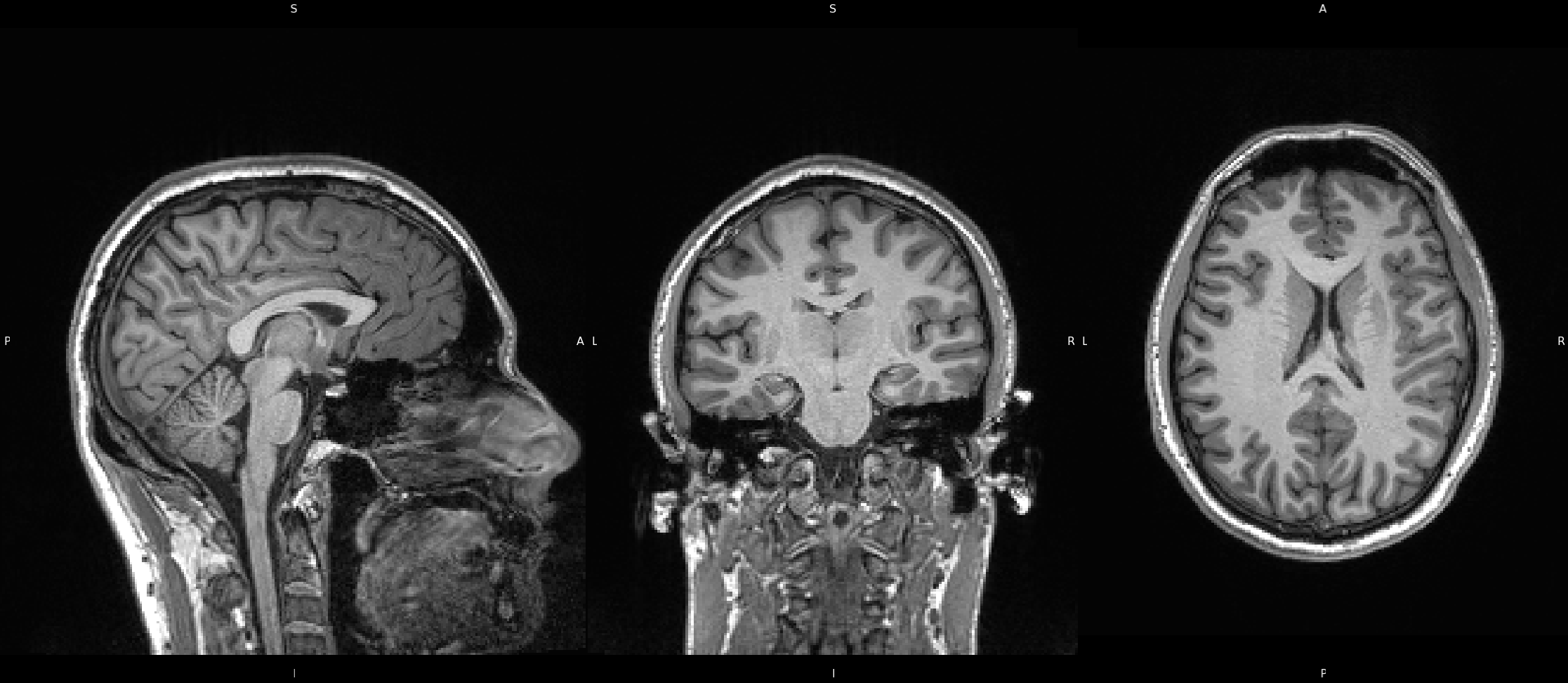
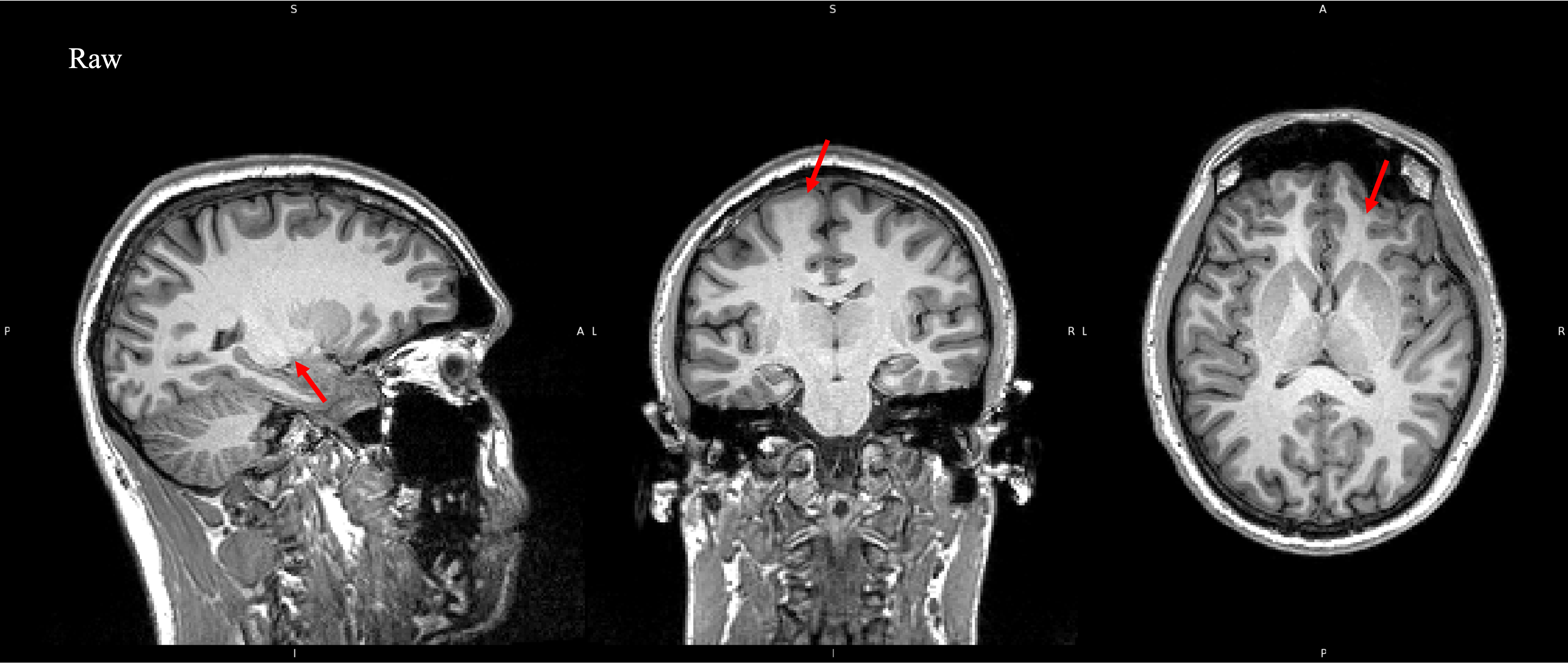
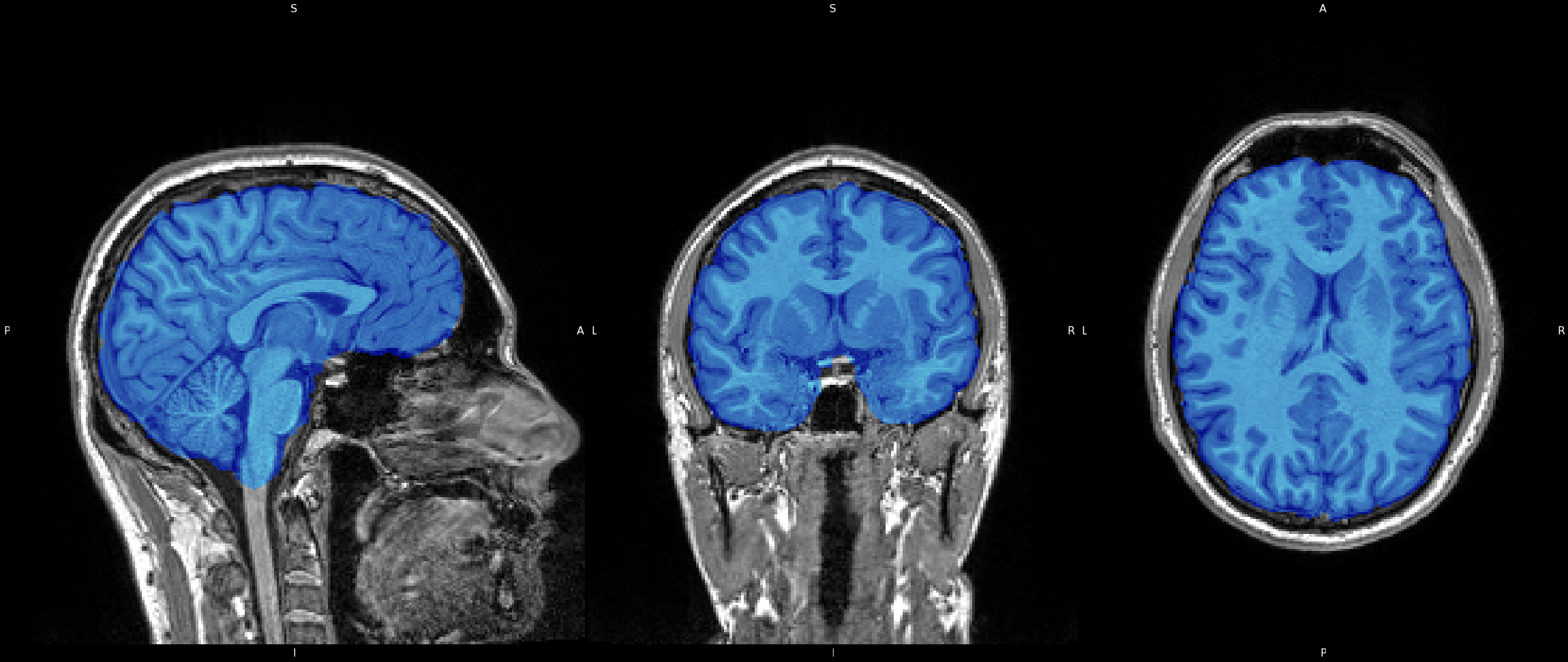
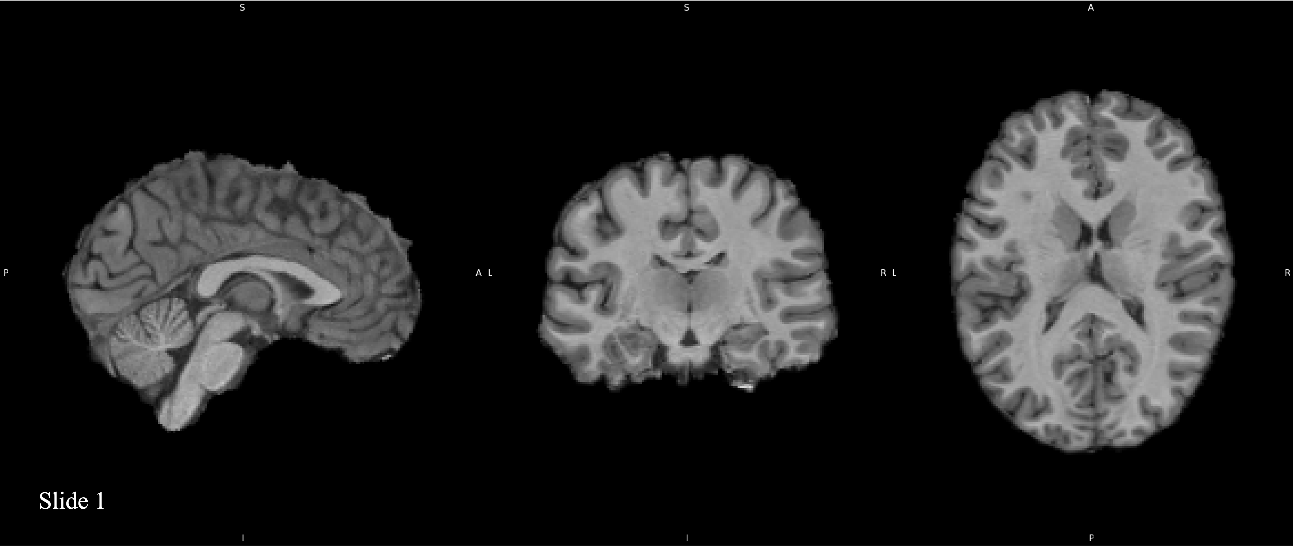
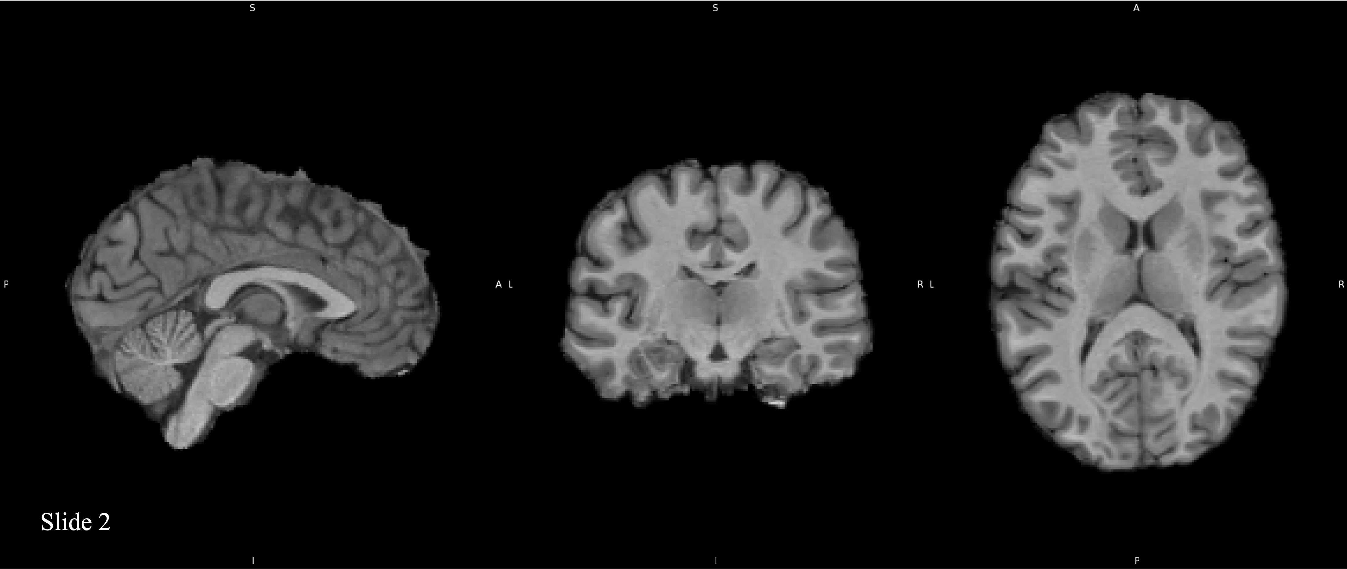
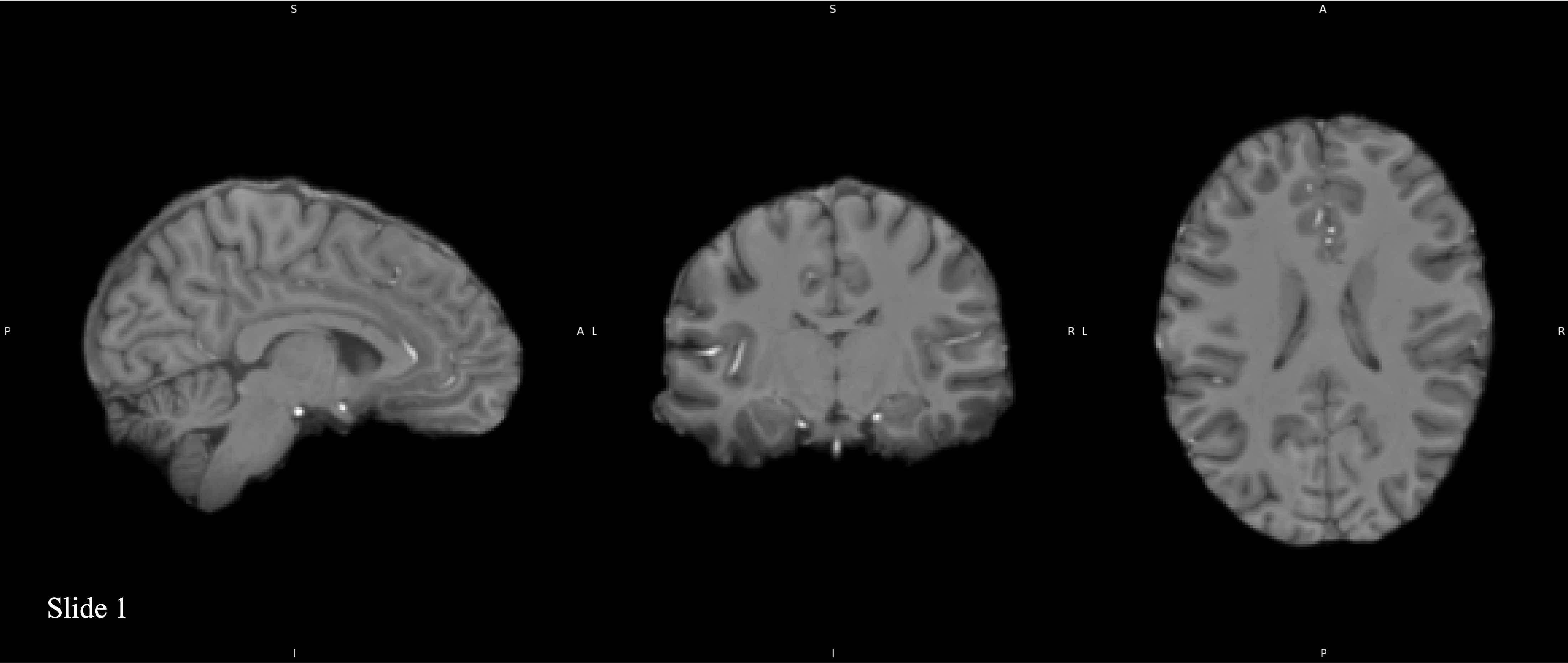
Here we have a T1 weighted image, collected from a 3T scanner. Image weighting and contrast is beyond the scope of this demonstration, but effectively this means that, in T1 images, areas of tissue containing fat will produce high signal and appear bright on the image, whereas areas of tissue containing water or Cerebrospinal Fluid (CSF) produce low signal and will appear dark on the image. Image resolution is not as good as in the 7T example, but the tissue intensity accross the image is more consistant than in the 7T. Some slight ringing artifacting can be seein in the frontal region in the sagittal image, which is a result of head motion but is reletivley insignifitant here. The skull, and other bits, are still present in the image, which we are not interested in and will be removed in a following step. Click below to view a video scrolling through each slice in the 3 different planes (Sagittal, Coronal, Axial).
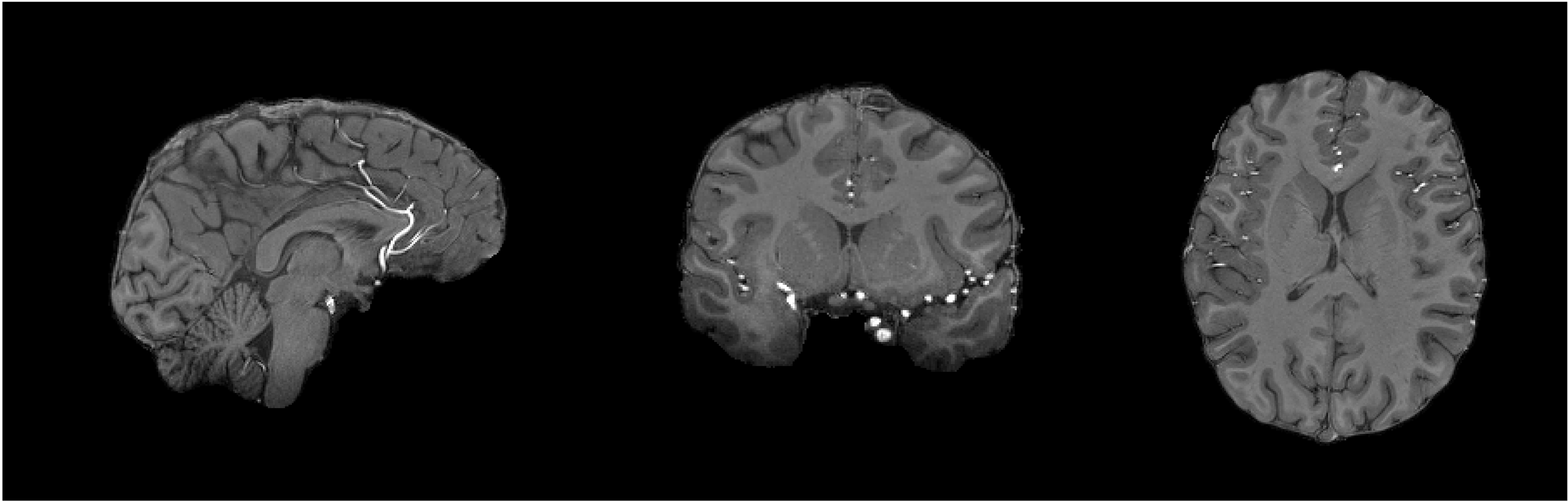
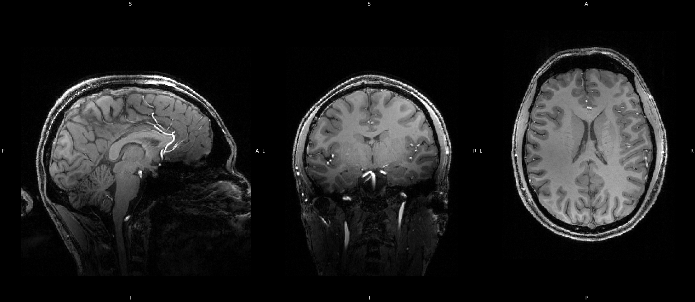
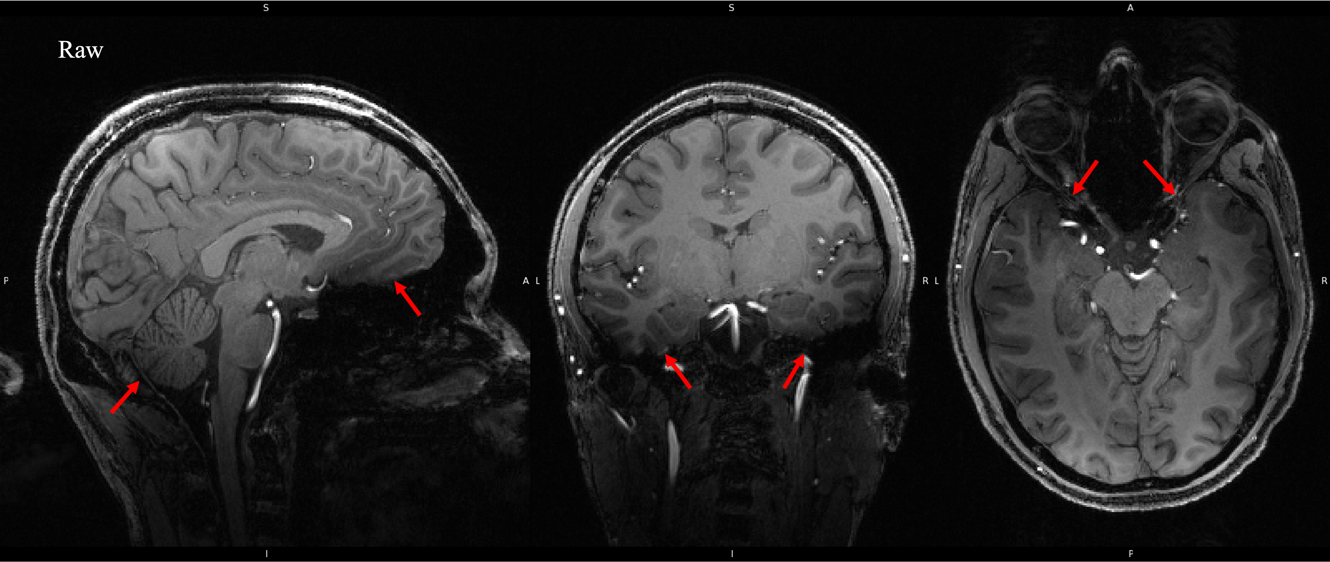
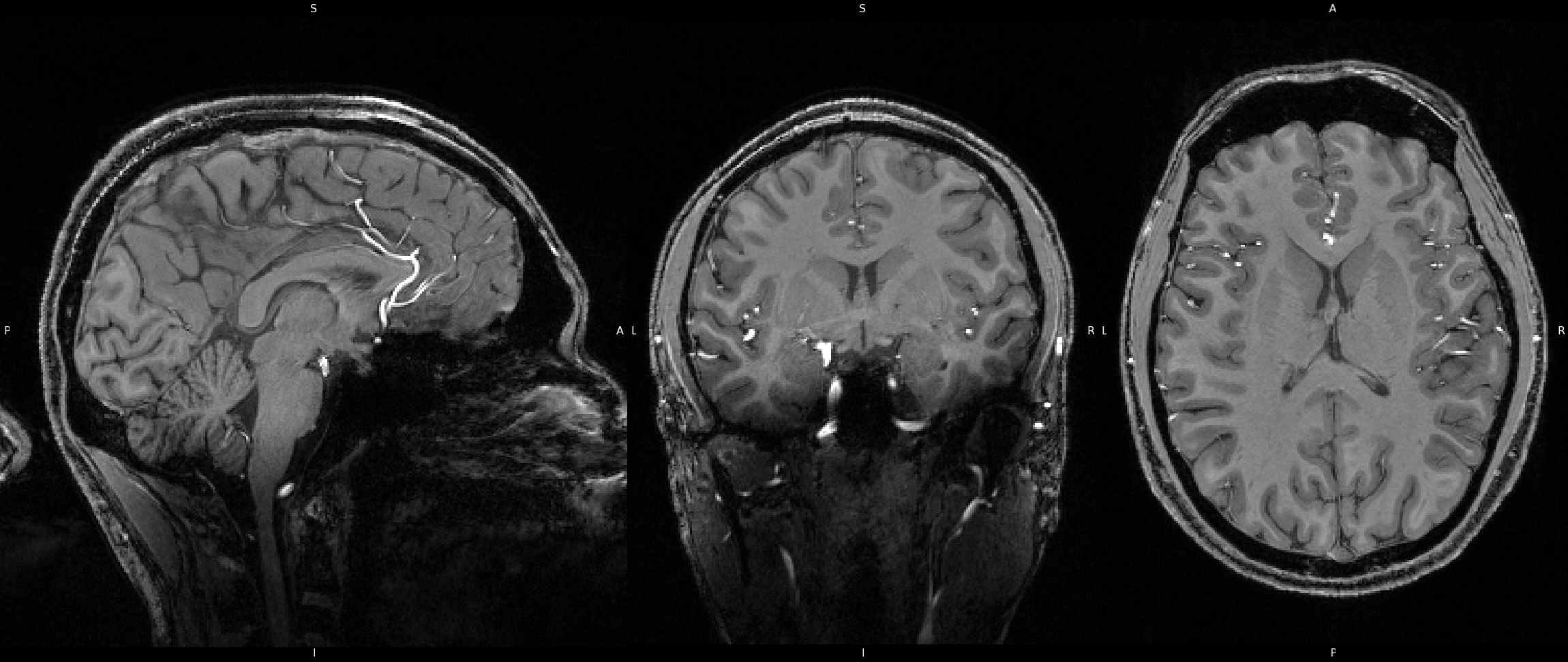
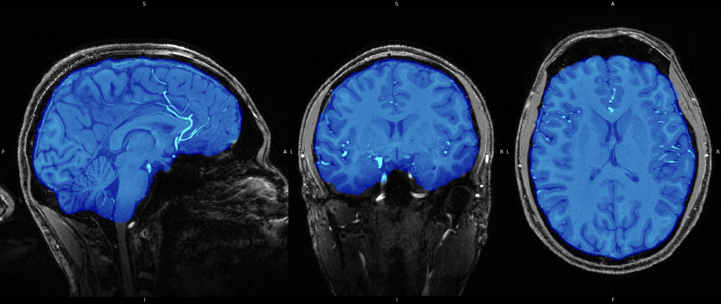
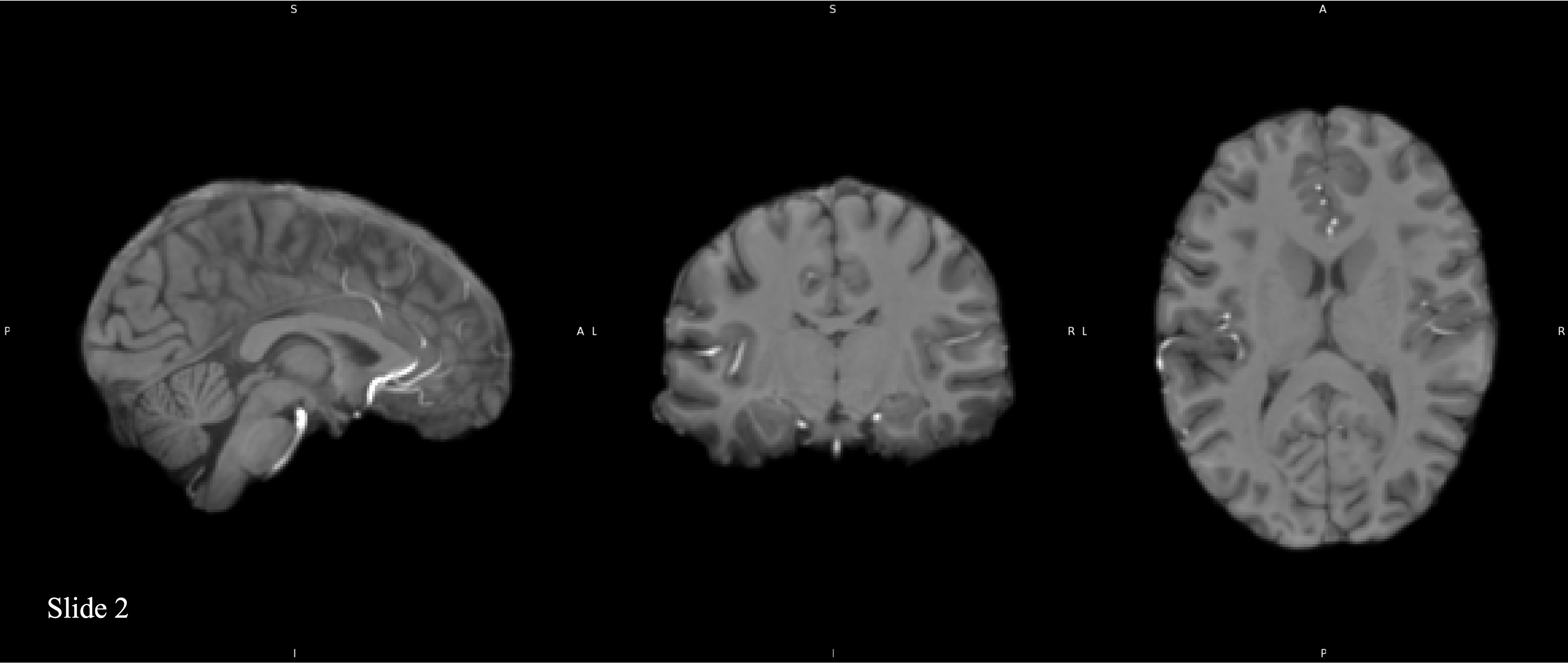
Here we have a T1 weighted image, collected from a 7T scanner. Since the image weighting is the same, the same areas will appear bright (fat) or dark (water/csf). However, due to the increased magnetic field strengh, we can achieve an image with higher resolution, which is apparent here. The drawback of this is magnetic susceptibility artifacting, which results in image intensity inconsistencies, such that areas will be brither or darker than they should. This can be seen here in the temporal areas of the coronal image, where the white matter tissue appears darker than in other areas of the brain. While the white matter and grey matter are still distingishable to us, this artifacting can cause issues in computer program processing tools where there might be a mis-classification of white matter as grey matter. Luckily, we can correct for these inhomogenieties which we will go over in the next step.
The magnetic field of a scanner should, in theory, be homogenious, but this is not the case. It is stronger in some areas and weaker in others.
This can lead to bias in signal intensity throughout an image. Areas where the magnetic field is stronger will produce stronger signal
than there should be, and vice versa. As a result some areas will appear brighter or darker than they should. This can be seen in the
example image below, particularly in areas where white matter boarders gray matter, (red arrows). This voxel intensity artifacting can cause
problems in processing tools and so we correct for it using Bias Field Correciton. Here I used N4ITKBiasFieldCorrection from
3D Slicer, and you can view the code down below. Before and after comparisons can be made by clicking on the example image below.
Click on the image to switch between the uncorrected and corrected images in order to see the differences. You'll notice that the signal
intensity in the corrected image is much more uniform and consistant between tissue types. The differences here are subtle, but can be significant
to processing tools which is why we need to correct for them, and are more obvious in the 7T image.
Click image to see results
As the strength of the magnetic field increases so does magnetic susceptibility artifacting. This is much more obvious here in the 7T image below.
Artifacting like this can cause problems in cortical segmentation and tissue classificaiton algorithms, which is why we want to correct for it.
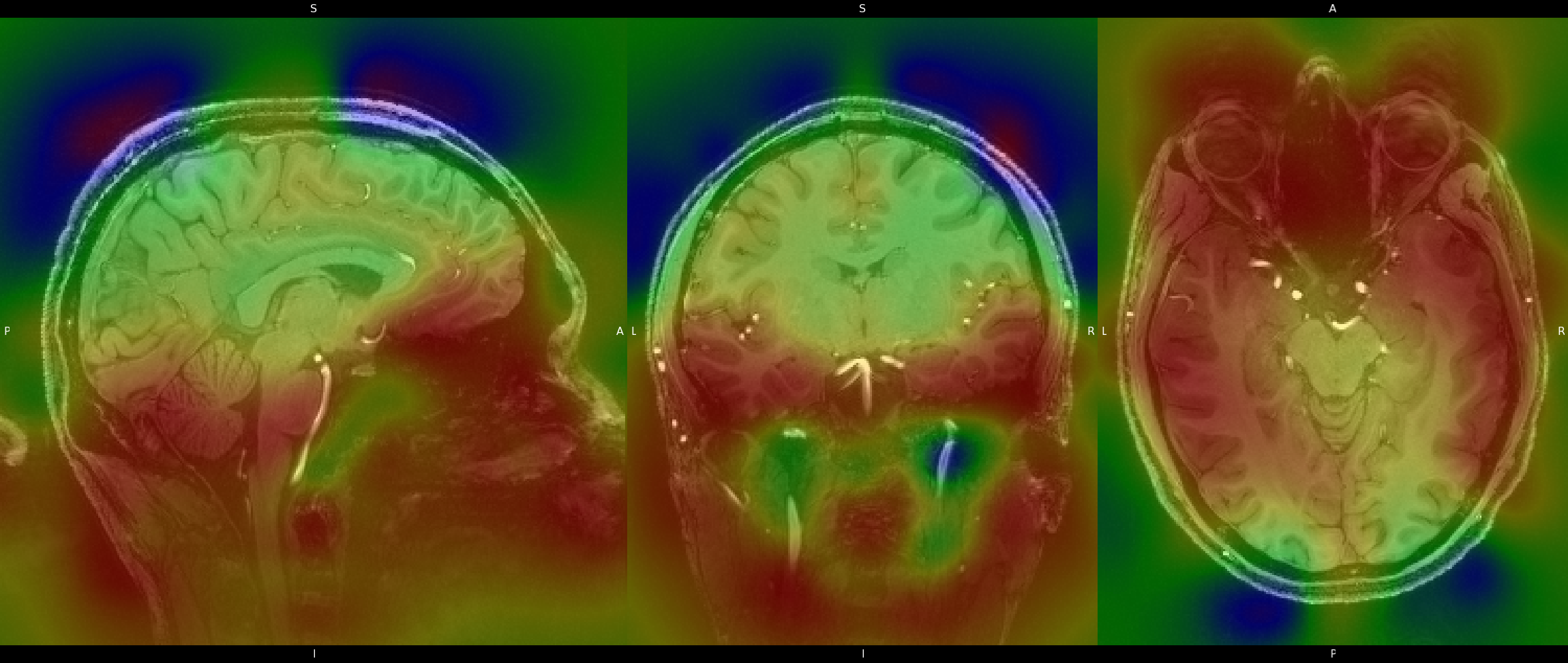
An example of the bias field using a color gradiant is provided below as well. Red signifies areas that suffered greater signal deterioration,
from inhomogenieties in the magnetic field. Again I use N4ITKBiasFieldCorrection to correct the biasing, and the code can be viewed
below. You can also click on the image to switch between the corrected and uncorrected images, to see the result of the correction.
Click image to see results
Because the brain is our primary interest here, we must isolate it from the non-important areas. Portions of the image, such as neck, eyes, nose, and skull are of no interest to us, and so we must remove them from the image. We do this because, similarly to Bias Field Correction, it will allow image processing algorithms to perform much smoother and quicker if these areas are not present in the image. Therefore we perform what is called "Brain Extraction". There are many tools available to do so, but here I use FMRIB's Software Lirbrary (FSL) Brain Extraction Toolkit (BET). Click on the image to see the image after running BET on the data. You can also view an overlay by clicking the overlay collapsable.
Click image to see results
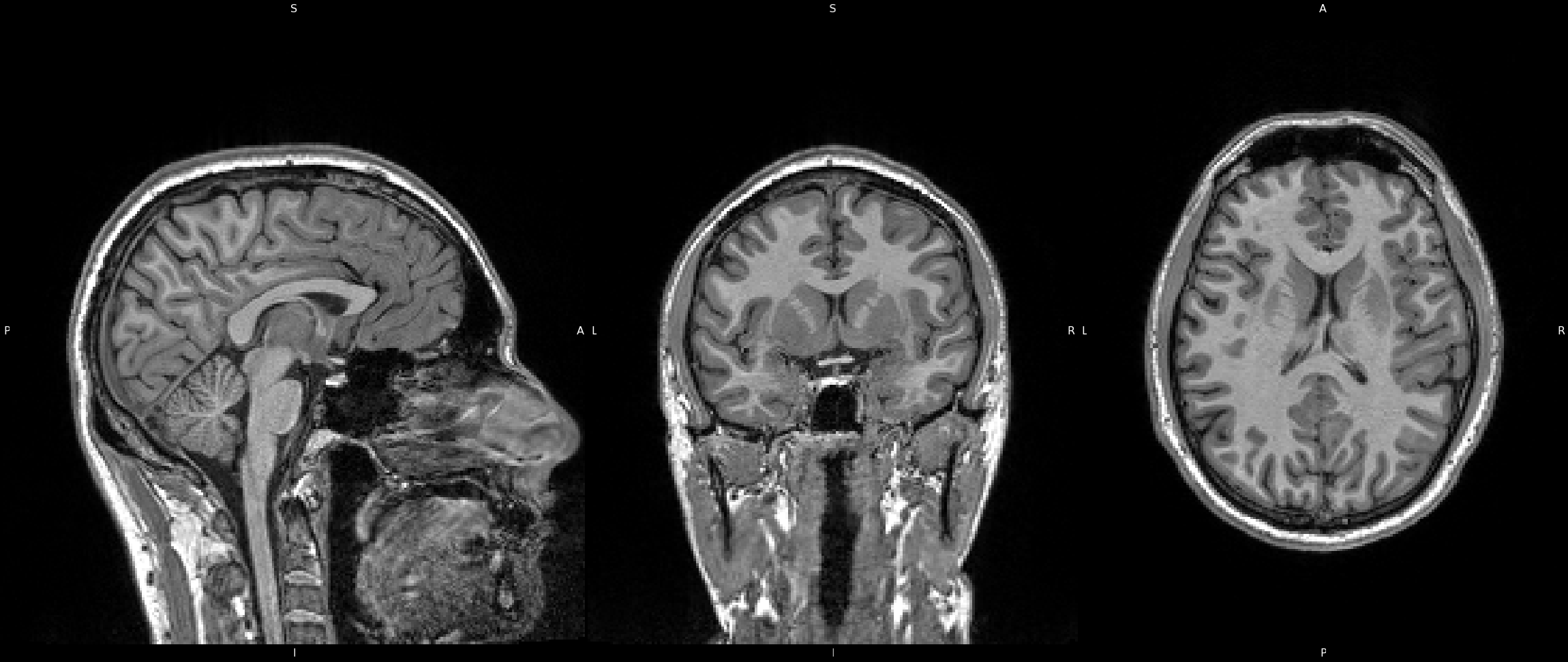
Brain Extraction was also run on the 7T image all the same using FSL's BET. Just as in the 3T image, BET does an excellent job of removing non-brain areas, and isolating brain tissue. You'll notice that the "-f" option uses a value of "0.3" instead of "0.4". The "-f" option adjusts the fractional intensity threshold, which basically controlls the outline the algorithm uses to isolate the brain. Larger values are more restrictive and will result in more areas being removed, whereas smaller values are more lenient and will result in less areas being removed. I chose the values here simply by trial and error and stuck with which option gave the best resultant image. You can also click on the image here to see the results of BET on the 7T image, as well as view the overlay by clicking the overlay collapsable.
Click image to see results
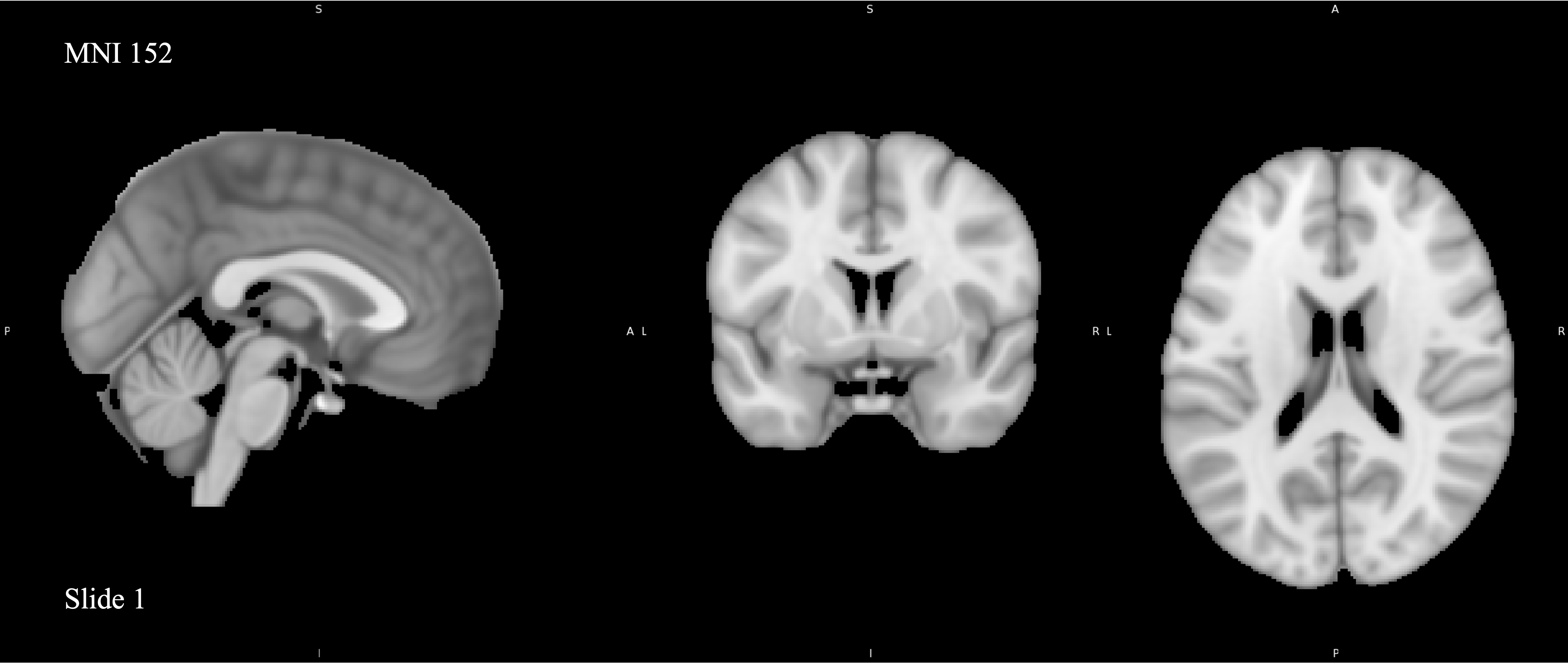
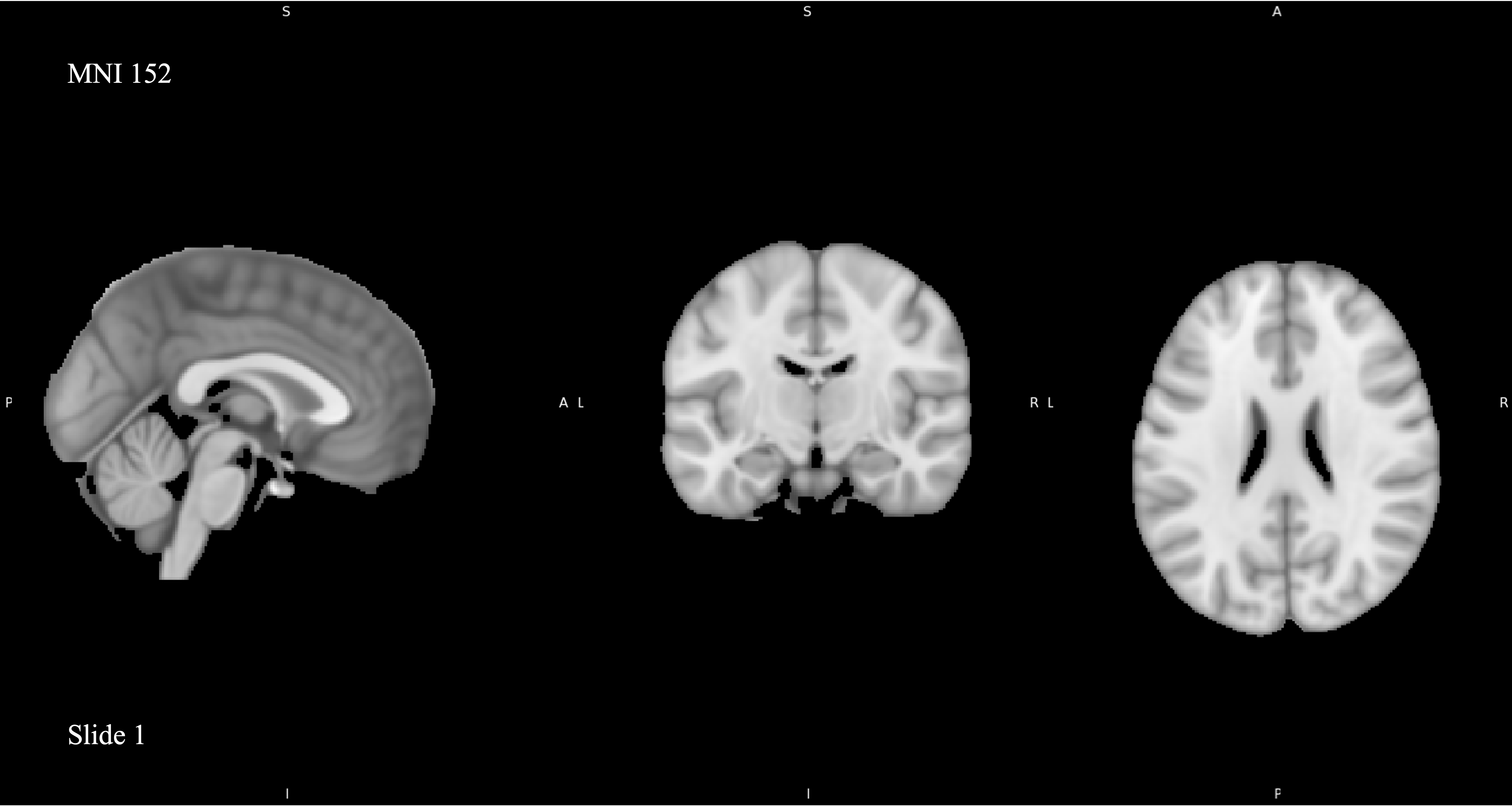
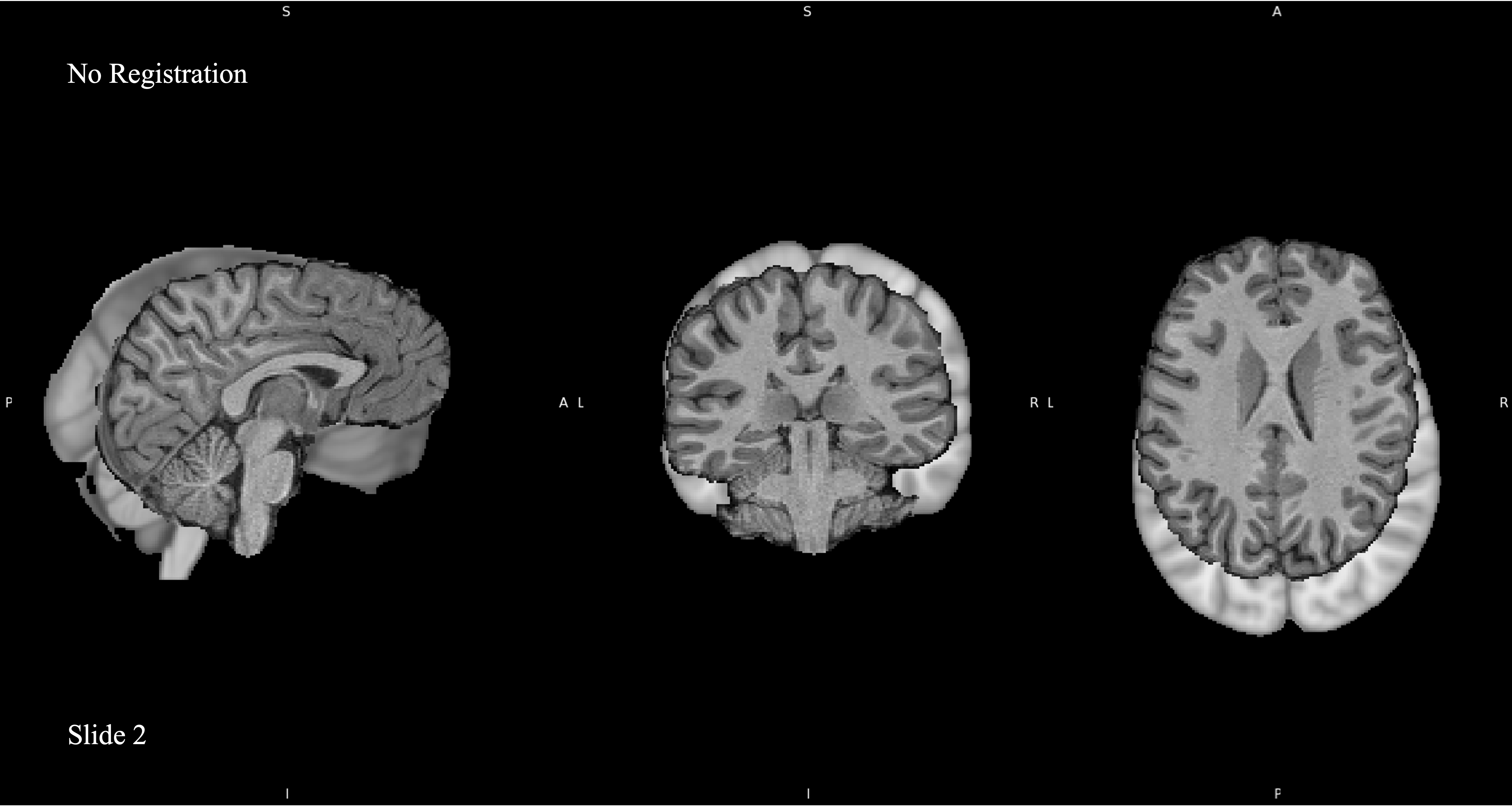
Before we can start making comparisons we need to perform one last pre-processing step, registration. Images from different sessions will be placed in a different "3D space" with different spacial coordinates, and so we must transform the images so that they are aligned anatomically. To do this I used FSL's Linear Image Registration Tool (FLIRT), via the GUI. FLIRT was run in 2 different ways, oncee using 6 degrees of freedom (DOF) Rigid body registration and again 12 DOF Affine registration. In both versions I used the MNI 152 atlas as the reference image, which is a template of 152 averaged brains and is the standard used for image registration.
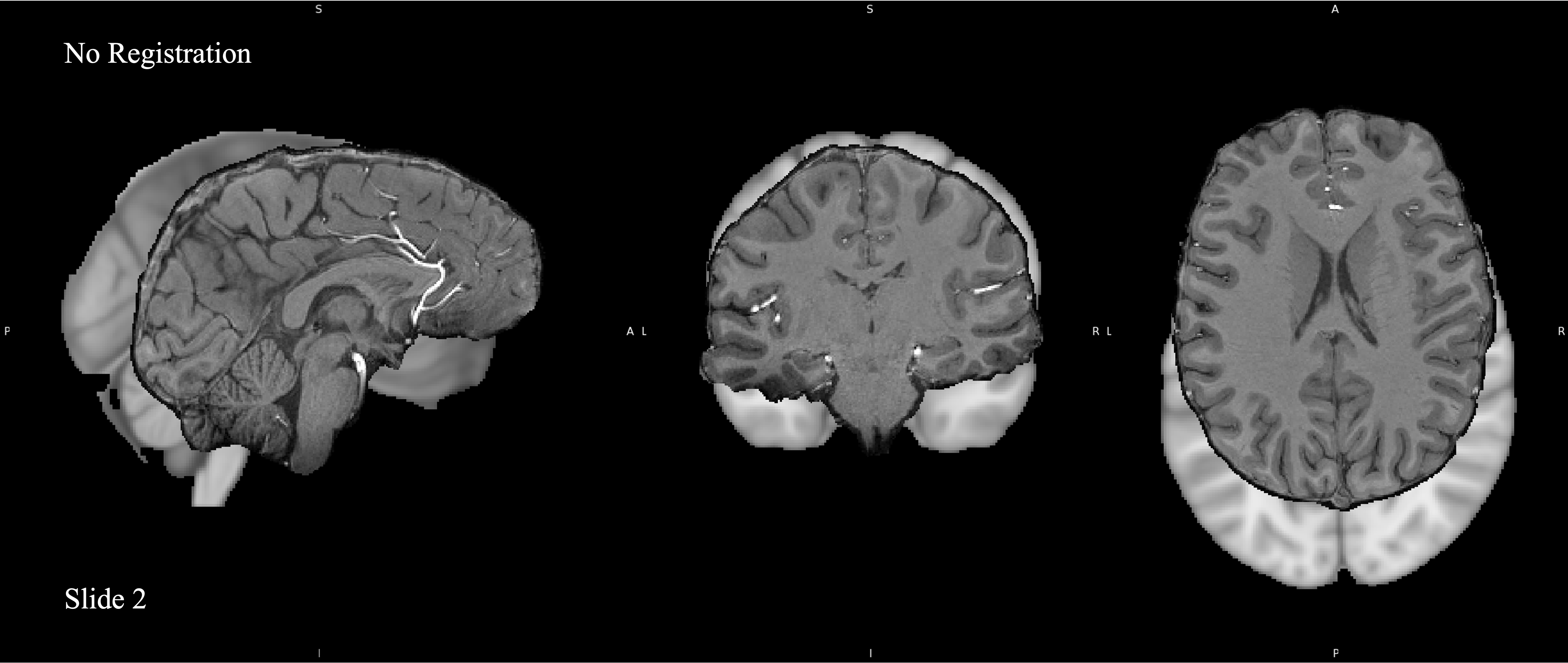
An example of the MNI 152 atlas can be seen in Slide 1 below. Click on the image to see the 3T image overlayed before registration. You can see how the 2 images are not aligned in the same space and that the overlaping tissue does not match anatomically. Hence why we must perform registration. The MNI atlas acts as an average for the general population, which is why we use it as the reference for the registration. Click the arrow to move to slide 2 and see the resutls of the 6 DOF registration.
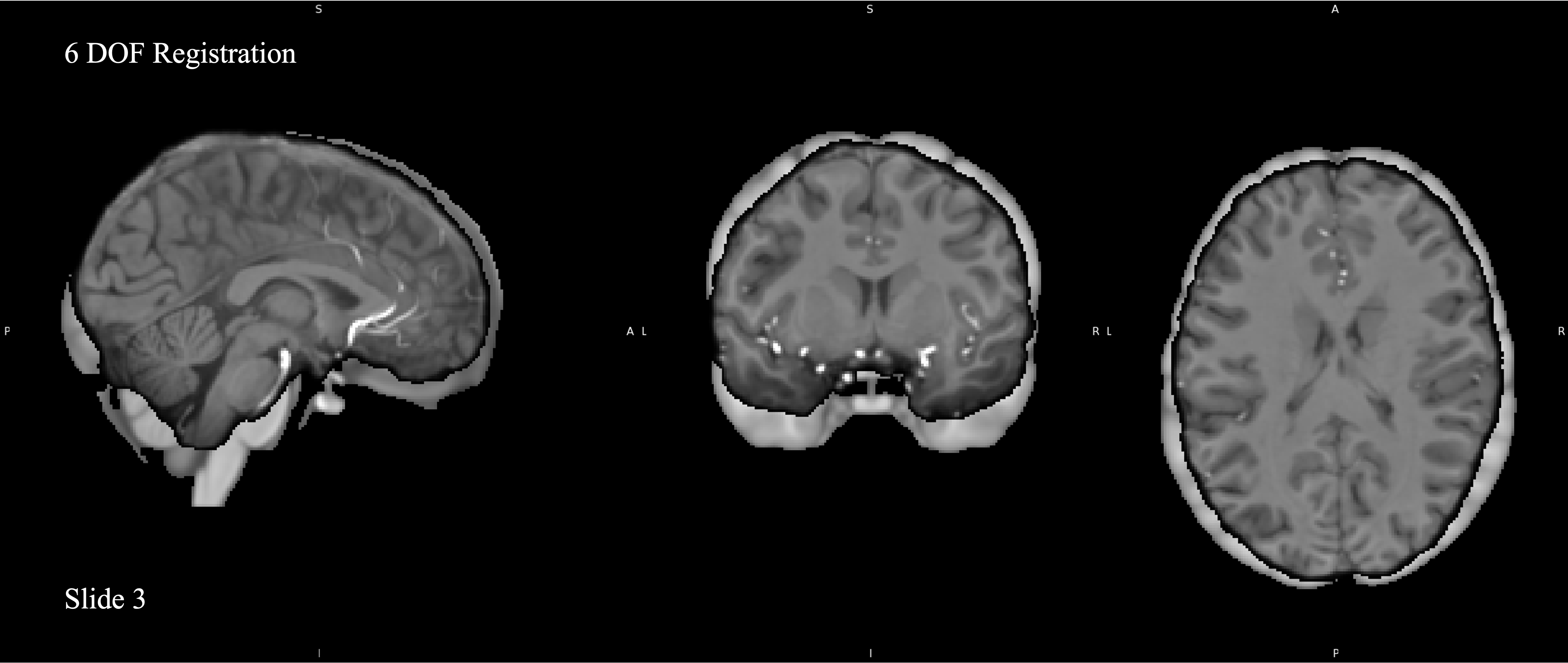
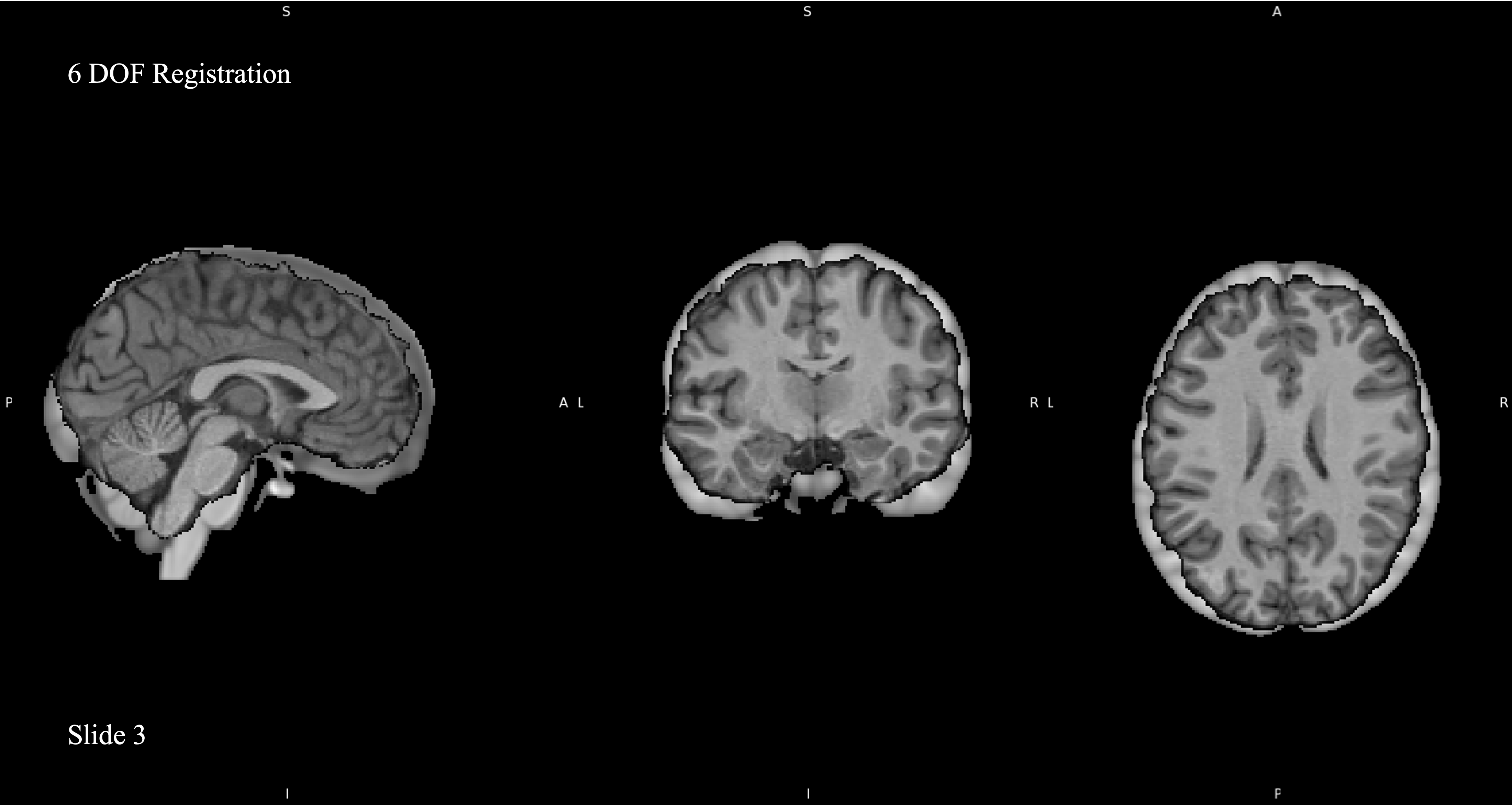
Here again we have the 3T overlay. Click on the image to see the results of the 6 DOF registration. Also refered to as a rigid body registration, this merely rotates and shifts the 3T image so that it roughly aligns with the MNI atlas, there is no re-sizing or shearing of the image. The reason for using a rigid body registration was to register the image to standard space while also preserving the true anatomy of the image for Tissue Classification and Segmentation.
Click on the image below to see the results of the 12 DOF Affine registration. You can see that the image gets blown up to match the MNI image. Along with rotating and shifting the image the Affine registration scales and warps the image so that it conformts to the MNI reference. The image is now fully aligned with the MNI reference and can use MNI coordinates for navigating and reporting findings. The purpose of the Affine registration was to fully align the image to MNI space for use as an underlay for Resting State fMRI ICA noise removal.
Registration for the 7T image was the same as for the 3T image. I used FSL's FLIRT, again using the GUI, aligning to the MNI 152 image for reference. Both kinds of registration, 6 DOF Rigid body and 12 DOF Affine, were also used here. Scroll through the slides below to see the results.
Here's where things get a bit more interesting. Tissue Classification is a process in which we segment the tissue types into individual parts, Grey Matter (GM), White Matter (WM), and Cerebrospinal Fluid (CSF). For this step I used FMRIB's Automated Segmentation Tool (FAST). This tool will first perform a "hard" segmentation where the tissue types will be defined dichotomously, as either fully belonging to a one tissue type or another. This is refered to as a binary segmentation and can be seen below in the first slide. However, this is an oversimplification of the true anatomy. Indeed there are many voxel in an image that are 100% one tissue type or another, but that is not the case for all voxels. There are many voxels that possess a mixture of tissue types, which is where the partial volume estimation (PVE) comes in. An example of a PVE map can be seen below in slide 2. Additionally, you can view the code I used to run the classificaiton, videos for both the "hard" segmentation and the PVE maps, as well as a calculation of the volume for each tissue type.
An example of the processed image is provided below. Click on the image to see the results of the "hard" segmentation. The image is colored so that the CSF appears Green, the Grey Matter appears Blue, and the White Matter appears Red. You'll notice that there is no gradual change in the coloring, they are either classified/colored as belonging to one or another. Hence why it's called a binary or "hard" segmentation.
Click on the image to see the results of the Partial Volume Estimation. The PVE maps are colored such that the Grey Matter (GM) ranges from a Cyan to Dark Blue, cyan being classified as 100% GM and dark blue being a mixture of pirmarily GM and one of the other two tissue types. Similarly the White Matter (WM) ranges from Yellow to Red, such that Yellow areas represent 100% pure WM and Red areas represent a mixture of mostly WM and one or more of the othe two tissue types. Lastly CSF is ranges from light to dark green, the ligher areas being pure CSF and the darker areas being a mixture.
There are little differences to mention between the 3T and 7T results. So I will use this to talk more about various other details about the methods I used and the process in general. For starters I used the "-N" option in my run of FAST, this prefents the tool from performing running bias field correction. Since I had already done this I didn't feel it necessary to do it again. As for the volume calculation, if I had more data I could use this to make comparisons between subjects or groups for differences in either Grey Matter or White Matter volume.
An example of the processed image is provided below. Click on the image to see the results of the "hard" segmentation. The image is colored so that the CSF appears Green, the Grey Matter appears Blue, and the White Matter appears Red. You'll notice that there is no gradual change in the coloring, they are either classified/colored as belonging to one or another. Hence why it's called a binary or "hard" segmentation.
Click on the image to see the results of the Partial Volume Estimation. The PVE maps are colored such that the Grey Matter (GM) ranges from a Cyan to Dark Blue, cyan being classified as 100% GM and dark blue being a mixture of pirmarily GM and one of the other two tissue types. Similarly the White Matter (WM) ranges from Yellow to Red, such that Yellow areas represent 100% pure WM and Red areas represent a mixture of mostly WM and one or more of the othe two tissue types. Lastly CSF is ranges from light to dark green, the ligher areas being pure CSF and the darker areas being a mixture.

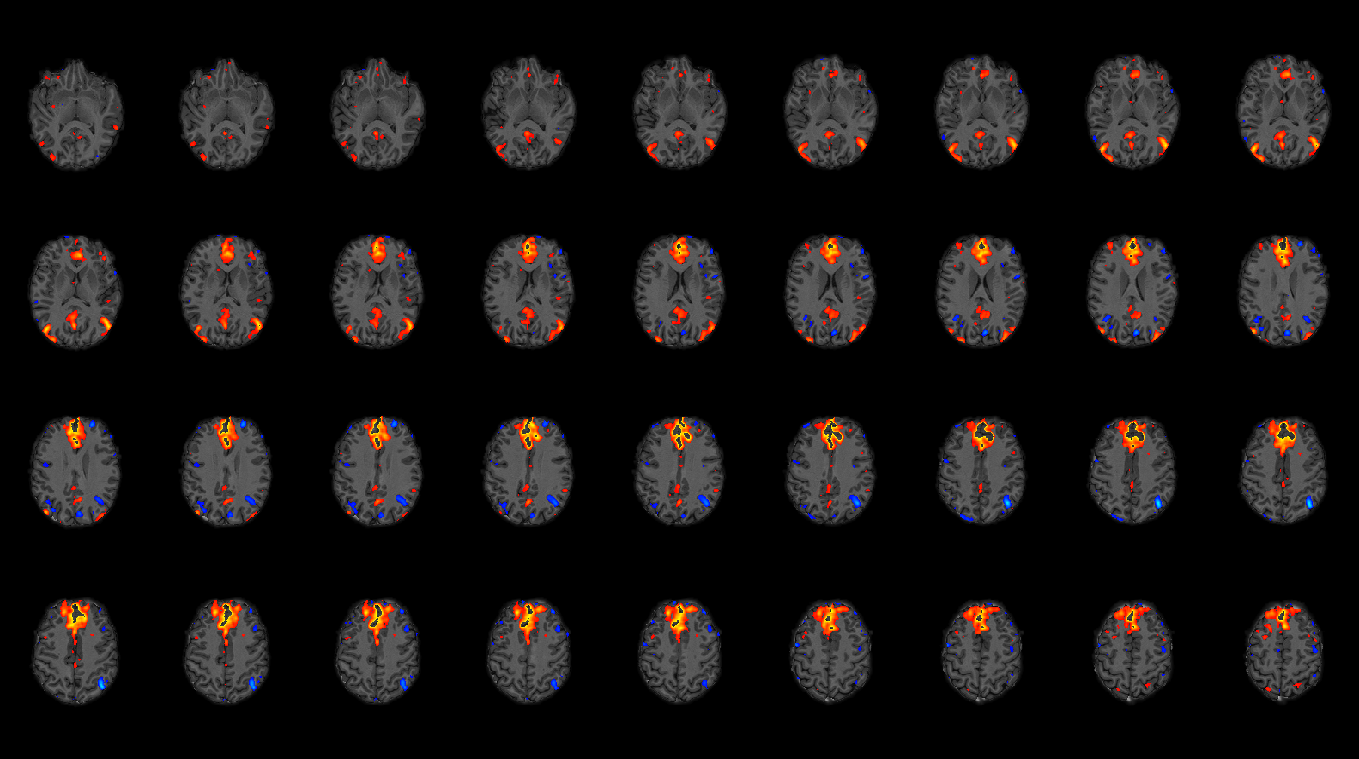
This section will present functional data collected on myslef at USC, specifically resting state data. Structural data was processed using the methods described in the Structural section (Skull Striping, Bias Field Correction, etc). Functional data was corrected for EPI distortions using Blip-Up and Blip-Down Field Maps following the Instructions provided by The Lewis Center for Neuroimaging at the University of Oregon. Both structural and functional data were registered to MNI space. An independent component analysis was run using FSL's MELODIC, and FSL's MELODIC viewer was used to label each Independent Component.
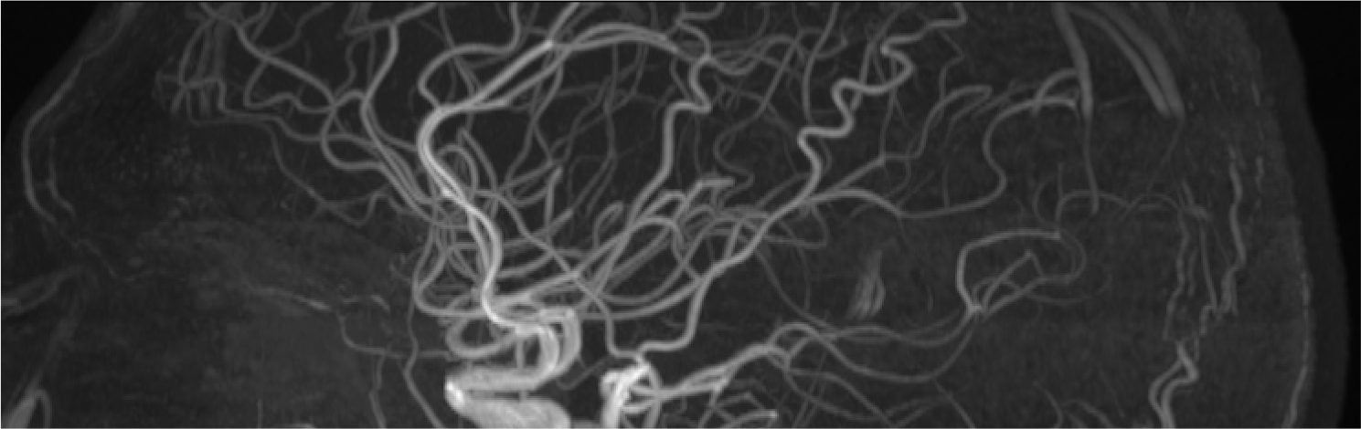
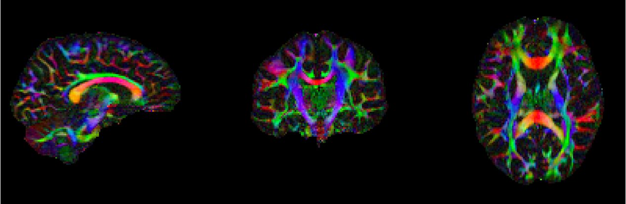
This section will present diffusion weighted data collected on myself at USC. Non-Diffusion weighted B0 images were prepared using FLS fslmerge, fslmaths, and topup. Diffusion Data was corrected for susceptibility distortions, EDDY currents, and movement using eddy. Fractional Anisotropy (FA) and Mean Diffusivity (MD) images were generated using fsl's dtifit, with which I was able to generate tensors. I was also able to use fsl to generate an FA skeleton that could be used for Tract-Based Spatial Statistics (TBSS). Lastly using DSI Studio, I was able to produce a estimated whole brain reconstruciton of the white matter architacture of my brain, seen on the right.